Comparison of more than 2 means with the AmericasBarometer

Introduction

In this section we will see how to construct confidence intervals of the mean using the data from the AmericasBarometer for more than two groups. For that, we will continue to use the last regional report “The Pulse of Democracy” for 2021 round, available here, and for the 2018/19 round, available here, where the main findings of the AmericasBarometer are presented. In both reports, one of the sections reports the results on support for electoral democracy by country. This type of plot is one of the most used with the AmericasBarometer data because it uses data for one wave to its limits, presenting a panoramic view of the region for a critical variable like support for democracy in all the countries in Latin America

About the dataset

The data we are going to use should be cited as follows: Source: AmericasBarometer by the Latin American Public Opinion Project (LAPOP), wwww.LapopSurveys.org. We can download the data freely here.

This section loads a trimmed database, originally in SPSS (.sav) format. This database is hosted in the “materials_edu” repository of the LAPOP account on GitHub. Using the library rio and the command import, you can import this database from this repository. In addition, the data from countries with codes less than or equal to 35 are selected, that is, the observations of the United States and Canada are eliminated.

library(rio)
lapop18 = import("https://raw.github.com/lapop-central/materials_edu/main/LAPOP_AB_Merge_2018_v1.0.sav")
lapop18 = subset(lapop18, pais<=35)

We also load the dataset for the 2021 round.

lapop21 = import("https://raw.github.com/lapop-central/materials_edu/main/lapop21.RData")
lapop21 = subset(lapop21, pais<=35)

Support for democracy by country 2021

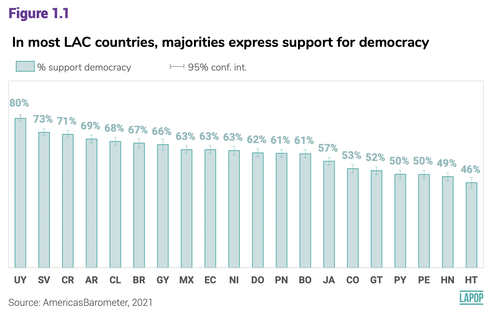
Figure 1.1 shows the percentage of citizens that supports democracy in each country. Each country bar includes the 95% confidence interval. The question in which is based this figure is: ING4. Changing the subject again, democracy may have problems, but it is better than any other form of government. To what extent do you agree or disagree with this statement? Respondents can answer in a 1-7 scale, where 1 means “Strongly disagree” and 7 “Strongly agree”.

To calculate these percentages, we hace to recode all answers between 5 and 7 as those who support democracy.

First, we have to define a new variable with this recodification that identifies supporters.

library(car)
lapop21$ing4r = car::recode(lapop21$ing4, "1:4=0; 5:7=100")
table(lapop21$ing4r)

## 
##     0   100 
## 20523 36240

To replicate Figure 1.1, we have to define a variable that identifies countries as a variable of type factor. For this, we calculate a new variable “paises” as factor with the command as.factor and we label it the the initials of each country, with the command levels, in the same way as it is shown in Figure 1.1.

lapop21$paises = as.factor(lapop21$pais)
levels(lapop21$paises) = c("ME", "GT", "SV", "HN", "NI",
                            "CR", "PN", "CO", "EC", "BO", "PE",
                            "PY", "CL", "UY", "BR", "AR", "DO",
                            "HT", "JA", "GY")
table(lapop21$paises)

## 
##   ME   GT   SV   HN   NI   CR   PN   CO   EC   BO   PE   PY   CL   UY   BR   AR 
## 2998 3000 3245 2999 2997 2977 3183 3003 3005 3002 3038 3004 2954 3009 3016 3011 
##   DO   HT   JA   GY 
## 3000 3088 3121 3011

Once done, we can use the library Rmisc` and the command summarySE`to calculate the means (that is, the percentages) of support for democracy in each country. This command also includes the standard deviation, the standard error and the confidence interval. We save this table in an object “df”.

library(Rmisc)
df = summarySE(data=lapop21, measurevar="ing4r", groupvar="paises", na.rm=T)
df

With this table “df” we can replicate Figure 1.1 using the library ggplot in the same way as previous sections show.

library(ggplot2)
fig1.1 <- ggplot(df, aes(x=reorder(paises, ing4r), y=ing4r))+
  geom_bar(width=0.5, fill="purple", colour="black", stat="identity")+
  geom_errorbar(aes(ymin=ing4r-ci, ymax=ing4r+ci), width=0.2)+
  geom_text(aes(label=paste(round(ing4r, 1), "%")), vjust=-1.5, size=2)+
  xlab("Country")+
  ylab("Support for democracy")
fig1.1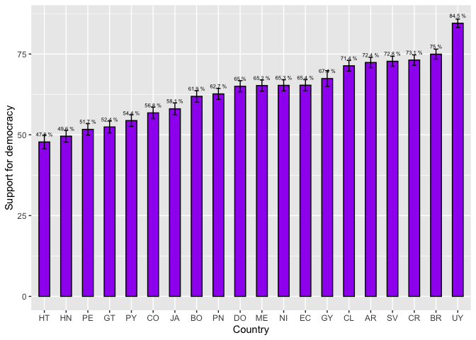

These results are not the same as those presented in Figure 1.1 because they do not include survey weights.

Support for democracy by country 2018/19

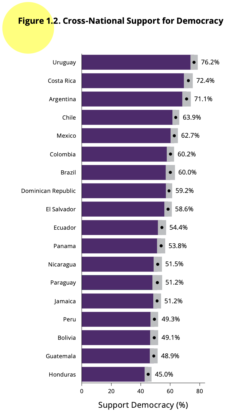
Figure 1.2 of the 2018/19 report shows the average support for electoral democracy for each of the 18 countries analyzed. It also presents the confidence intervals for each country, in the form of a gray bar, which indicates the lower and upper range of this interval, with a dot indicating the mean value.

To reproduce the data in this graph, you first have to recode the variable, in the same way as was done in the section about confidence intervals.

library(car)
lapop18$ing4r = car::recode(lapop18$ing4, "1:4=0; 5:7=100")
table(lapop18$ing4r)

## 
##     0   100 
## 11463 15623

When the database is imported, the variables are defined as numerical, and many of them are factors, such as the variable “pais”. In order to evaluate support for democracy by country, a new variable “paises” is defined as a factor and labeled.

lapop18$paises = as.factor(lapop18$pais)
levels(lapop18$paises) = c("Mexico", "Guatemala", "El Salvador", "Honduras", "Nicaragua",
                            "Costa Rica", "Panama", "Colombia", "Ecuador", "Bolivia", "Peru",
                            "Paraguay", "Chile", "Uruguay", "Brazil", "Argentina", 
                           "Dominican Republic", "Jamaica")
table(lapop18$paises)

## 
##             Mexico          Guatemala        El Salvador           Honduras 
##               1580               1596               1511               1560 
##          Nicaragua         Costa Rica             Panama           Colombia 
##               1547               1501               1559               1663 
##            Ecuador            Bolivia               Peru           Paraguay 
##               1533               1682               1521               1515 
##              Chile            Uruguay             Brazil          Argentina 
##               1638               1581               1498               1528 
## Dominican Republic            Jamaica 
##               1516               1513

With these variables, we create a new dataframe with the data on the average support for democracy for each country (which is the percentage of citizens that support democracy), with the data to build the confidence intervals. For this we use the command summarySE which is part of the library Rmisc. These data are saved in the dataframe “df2”.

library(Rmisc)
df2 = summarySE(data=lapop18, measurevar="ing4r", groupvar="paises", na.rm=T)
df2

With this new dataframe, a graph similar to Figure 1.2 of the report is constructed. It must be taken into account that some percentages are not similar to those shown in the report because this code does not include survey weights.

For the plot construction we use the library ggplot2. The command ggplot first requires you to specify the dataframe you are working with, which in this case is “df”. Next, the “aesthetics” of the graph are defined with the aes specification, indicating what information to include on each axis. By default the bars are vertical, so the “paises” variable is defined on the X axis, but the reorder specification is used to indicate that the bars do not follow the alphabetical order of the “countries” variable but rather are ordered by the values of the variable “ing4r”. In the Y axis, the variable “ing4r” is defined, which will mark the height of the bar.

Once the axes are defined, the command geom_bar is used to indicate that we want to create a bar chart. Within this command we specify the width, the internal color, the border color and, above all, that the data from the dataframe “df2” is used as it appears, with the specification stat="identity".

In addition to the bar, we add goem_errorbar to include the error bars that mark the limits of the confidence intervals. This layer also requires an aes aesthetic where the lower (ymin=ing4r-ci) and upper bounds are defined (ymax=ing4r+ci).

The specification geom_text is used to add the data labels to each bar. This specification requires an aes aesthetic where it is defined that the “ing4r” data will be used, but rounded to 1 decimal place and with the “%” symbol. We adjust the position of the label with hjust and the size of the label with size.

Finally, it is indicated that the X axis does not have a label and that the Y axis is named “Support for democracy according to countries. The coord_flip() specification is used to rotate the graph 90 degrees and present the horizontal bars.

library(ggplot2)
fig1.2 <- ggplot(df2, aes(x=reorder(paises, ing4r), y=ing4r))+
  geom_bar(width=0.5, fill="purple", colour="black", stat="identity")+
  geom_errorbar(aes(ymin=ing4r-ci, ymax=ing4r+ci), width=0.2)+
  geom_text(aes(label=paste(round(ing4r, 1), "%")), hjust=-0.8, size=2)+
  xlab("")+
  ylab("Support for democracy by country")+
  coord_flip()
fig1.2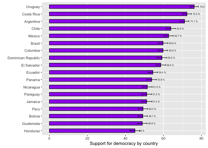

This type of graph is widely used in the AmericasBarometer reports and others produced by LAPOP. This graph shows the average value of support for democracy in each country and a bar with 95% confidence intervals. In this way, a visual comparison can be made between countries to see where there might be statistically significant differences. When the confidence intervals of two countries overlap, we may say that there is a difference in the population average of support for democracy. On the other hand, if the confidence intervals do not overlap, we may say that there is a population difference in the average support for democracy among the countries.

If, for example, the average support for democracy is compared between Uruguay (76.2%) and Costa Rica (72.4%), the countries at the top of the ranking, we may say that the population averages of both countries are not different, since the confidence intervals overlap. On the contrary, if Argentina (71.1%) and Chile (63.9) are compared, we may say that the population average of support for democracy in Argentina is greater than the equivalent in Chile, since both confidence intervals do not overlap.

However, this visual comparison is for reference, because to find out if there are statistically significant differences among countries (or between a couple of countries), a statistical test must be carried out. In the section on comparison of 2 means, a t-test was used to compare two groups. This same test could be used to compare whether the differences in the sample means between two countries can be extrapolated, but it does not help if one wanted to have a general comparison between this entire group of countries, or it would be very cumbersome to have to make multiple comparisons for each country pair.

In order to have that general picture and, in turn, be able to evaluate the pairings, another statistical test can be used.

ANOVA test

The ANOVA test is used to compare the mean of a numerical variable between groups of a variable type factor. In this case, we use the ANOVA test with a dummy variable, coded as 0-1, so that the mean equals the proportion.

This test is based on the F distribution and proposes the following null hypothesis for the comparison of a numerical variable X between n groups of the factor variable.

\[ H0: \mu_{x1} = \mu_{x2} = \mu_{x1} =...= \mu_{xn} \]

The alternative hypothesis it proposes is that at least one population mean of a group is different.

Evaluating means using ANOVA

The command aov performs analysis of variance with a numeric variable and a variable of type factor with more than 2 groups. This test is saved in an object called “anova” and the results are then described with the command summary.

For example, for the comparisons among countries in the 2021 report.

anova1 = aov(lapop21$ing4r~ lapop21$paises)
summary(anova1)

##                   Df    Sum Sq Mean Sq F value Pr(>F)    
## lapop21$paises    19   5043583  265452   119.6 <2e-16 ***
## Residuals      56743 125984290    2220                   
## ---
## Signif. codes:  0 '***' 0.001 '**' 0.01 '*' 0.05 '.' 0.1 ' ' 1
## 3898 observations deleted due to missingness

The value of the F test statistic is 119.6, with a corresponding very small p-value. Since this value of the p-value is less than 0.05, the null hypothesis can be rejected and we can affirm that at least one population mean is different. The ANOVA test does not tell us which means are different.

To find out which means are different, we have to evaluate the different pairings to find out the differences in each pair. This detail can be calculated with a post-hoc test called Tukey’s Test. In R this test can be run with the command TukeyHSD.

In this case there are many pairings because there are many countries. In each pairing there is the value of the difference of the variable “ing4r” between the 2 countries, as well as the lower and upper limit of this difference. The adjusted p-value (“p adj”) must be evaluated to know if the difference in support for democracy between these two countries is statistically significant and can be extrapolated to the population.

For example, Figure 1,1 shows that confidence intervals of support for democracy for Uruguay and El Salvador do not overlap, so we may say there is a statistically significant differenfce. Tukey`s test indicates that the p-value for this pairing is lower than 0.05, so we can confidently affirm that there is a difference in the population.

Figure 1.1 also shows that the confidence intervals for El Salvador and Costa Rica overlap, so we cannot say if there is a difference. Tukey`s test shows that this pairing reports a p-value closer to 1, higher than 0.05, so we cannot conclude that there is a statistically significant difference between these two countries.

TukeyHSD(anova1)

##   Tukey multiple comparisons of means
##     95% family-wise confidence level
## 
## Fit: aov(formula = lapop21$ing4r ~ lapop21$paises)
## 
## $`lapop21$paises`
##               diff          lwr           upr     p adj
## GT-ME -12.81110639 -17.21014734  -8.412065438 0.0000000
## SV-ME   7.51472777   3.23440052  11.795055007 0.0000001
## HN-ME -15.65991103 -20.03954846 -11.280273609 0.0000000
## NI-ME   0.06891815  -4.28488763   4.422723926 1.0000000
## CR-ME   7.89327831   3.52874562  12.257811001 0.0000000
## PN-ME  -2.58426407  -6.87771869   1.709190547 0.8399056
## CO-ME  -8.45440523 -12.80894488  -4.099865590 0.0000000
## EC-ME   0.11207218  -4.23408021   4.458224564 1.0000000
## BO-ME  -3.34744169  -7.70603319   1.011149820 0.4118048
## PE-ME -13.55648653 -17.88620050  -9.226772555 0.0000000
## PY-ME -10.84138024 -15.20442232  -6.478338170 0.0000000
## CL-ME   6.12046554   1.74691370  10.494017378 0.0001281
## UY-ME  19.28089777  14.93583101  23.625964536 0.0000000
## BR-ME   9.71404137   5.37186027  14.056222482 0.0000000
## AR-ME   7.13269126   2.78906902  11.476313499 0.0000011
## DO-ME  -0.22184272  -4.58899259   4.145307157 1.0000000
## HT-ME -17.45444100 -22.19729333 -12.711588678 0.0000000
## JA-ME  -7.19113997 -11.60694748  -2.775332452 0.0000015
## GY-ME   2.16117887  -3.26565130   7.588009046 0.9977259
## SV-GT  20.32583415  16.00919456  24.642473747 0.0000000
## HN-GT  -2.84880465  -7.26393772   1.566328428 0.7442009
## NI-GT  12.88002453   8.49051421  17.269534855 0.0000000
## CR-GT  20.70438470  16.30423450  25.104534888 0.0000000
## PN-GT  10.22684232   5.89718544  14.556499191 0.0000000
## CO-GT   4.35670115  -0.03353706   8.746939370 0.0545886
## EC-GT  12.92317856   8.54125927  17.305097854 0.0000000
## BO-GT   9.46366470   5.06940754  13.857921863 0.0000000
## PE-GT  -0.74538014  -5.11099570   3.620235415 1.0000000
## PY-GT   1.96972614  -2.42894550   6.368397787 0.9904296
## CL-GT  18.93157192  14.52247544  23.340668407 0.0000000
## UY-GT  32.09200416  27.71116163  36.472846690 0.0000000
## BR-GT  22.52514776  18.14716731  26.903128216 0.0000000
## AR-GT  19.94379765  15.56438784  24.323207453 0.0000000
## DO-GT  12.58926367   8.18651747  16.992009871 0.0000000
## HT-GT  -4.64333462  -9.41898371   0.132314478 0.0683755
## JA-GT   5.61996642   1.16895169  10.070981147 0.0013071
## GY-GT  14.97228526   9.51676862  20.427801901 0.0000000
## HN-SV -23.17463880 -27.47150278 -18.877774816 0.0000000
## NI-SV  -7.44580962 -11.71634131  -3.175277933 0.0000001
## CR-SV   0.37855054  -3.90291670   4.660017785 1.0000000
## PN-SV -10.09899184 -14.30797849  -5.890005180 0.0000000
## CO-SV -15.96913300 -20.24041286 -11.697853141 0.0000000
## EC-SV  -7.40265559 -11.66538437  -3.139926804 0.0000001
## BO-SV -10.86216945 -15.13758008  -6.586758824 0.0000000
## PE-SV -21.07121429 -25.31718170 -16.825246888 0.0000000
## PY-SV -18.35610801 -22.63605570 -14.076160316 0.0000000
## CL-SV  -1.39426223  -5.68492323   2.896398772 0.9998649
## UY-SV  11.76617001   7.50454810  16.027791917 0.0000000
## BR-SV   2.19931361  -2.05936610   6.457993321 0.9564240
## AR-SV  -0.38203651  -4.64218560   3.878112585 1.0000000
## DO-SV  -7.73657048 -12.02070565  -3.452435315 0.0000000
## HT-SV -24.96916877 -29.63569471 -20.302642835 0.0000000
## JA-SV -14.70586773 -19.03959270 -10.372142762 0.0000000
## GY-SV  -5.35354889 -10.71380092   0.006703139 0.0507278
## NI-HN  15.72882918  11.35876470  20.098893661 0.0000000
## CR-HN  23.55318934  19.17243776  27.933940925 0.0000000
## PN-HN  13.07564696   8.76570597  17.385587955 0.0000000
## CO-HN   7.20550580   2.83471019  11.576301415 0.0000010
## EC-HN  15.77198321  11.40954360  20.134422823 0.0000000
## BO-HN  12.31246935   7.93763693  16.687301769 0.0000000
## PE-HN   2.10342451  -2.24263830   6.449487309 0.9773844
## PY-HN   4.81853079   0.43926431   9.197797274 0.0142698
## CL-HN  21.78037657  17.39063916  26.170113978 0.0000000
## UY-HN  34.94080881  30.57945077  39.302166850 0.0000000
## BR-HN  25.37395241  21.01546923  29.732435581 0.0000000
## AR-HN  22.79260229  18.43268338  27.152521210 0.0000000
## DO-HN  15.43806832  11.05470924  19.821427396 0.0000000
## HT-HN  -1.79452997  -6.55231170   2.963251759 0.9988893
## JA-HN   8.46877107   4.03693231  12.900609828 0.0000000
## GY-HN  17.82108991  12.38120714  23.260972675 0.0000000
## CR-NI   7.82436016   3.46943362  12.179286707 0.0000000
## PN-NI  -2.65318222  -6.93687130   1.630506864 0.8040200
## CO-NI  -8.52332338 -12.86823478  -4.178411978 0.0000000
## EC-NI   0.04315403  -4.29335149   4.379659554 1.0000000
## BO-NI  -3.41635983  -7.76533207   0.932612403 0.3668110
## PE-NI -13.62540467 -17.94543508  -9.305374272 0.0000000
## PY-NI -10.91029839 -15.26373103  -6.556865753 0.0000000
## CL-NI   6.05154739   1.68758184  10.415512937 0.0001607
## UY-NI  19.21197963  14.87656214  23.547397111 0.0000000
## BR-NI   9.64512323   5.31259782  13.977648630 0.0000000
## AR-NI   7.06377311   2.72980337  11.397742858 0.0000014
## DO-NI  -0.29076086  -4.64831036   4.066788632 1.0000000
## HT-NI -17.52335915 -22.25737307 -12.789345233 0.0000000
## JA-NI  -7.26005811 -11.66637127  -2.853744961 0.0000010
## GY-NI   2.09226073  -3.32684670   7.511368155 0.9984831
## PN-CR -10.47754238 -14.77213351  -6.182951246 0.0000000
## CO-CR -16.34768354 -20.70334376 -11.992023322 0.0000000
## EC-CR  -7.78120613 -12.12848126  -3.433931006 0.0000000
## BO-CR -11.24071999 -15.60043103  -6.881008953 0.0000000
## PE-CR -21.44976484 -25.78060581 -17.118923863 0.0000000
## PY-CR -18.73465855 -23.09881902 -14.370498085 0.0000000
## CL-CR  -1.77281277  -6.14748032   2.601854776 0.9971565
## UY-CR  11.38761947   7.04142968  15.733809247 0.0000000
## BR-CR   1.82076307  -2.52254181   6.164067938 0.9956520
## AR-CR  -0.76058705  -5.10533268   3.584158583 1.0000000
## DO-CR  -8.11512103 -12.48338824  -3.746853810 0.0000000
## HT-CR -25.34771931 -30.09160049 -20.603838135 0.0000000
## JA-CR -15.08441828 -19.50133082 -10.667505728 0.0000000
## GY-CR  -5.73209943 -11.15982881  -0.304370060 0.0253704
## CO-PN  -5.87014116 -10.15457612  -1.585706207 0.0002154
## EC-PN   2.69633625  -1.57957394   6.972246438 0.7789850
## BO-PN  -0.76317761  -5.05173067   3.525375439 1.0000000
## PE-PN -10.97222246 -15.23142314  -6.713021773 0.0000000
## PY-PN  -8.25711617 -12.55019240  -3.964039942 0.0000000
## CL-PN   8.70472961   4.40097275  13.008486465 0.0000000
## UY-PN  21.86516184  17.59035512  26.139968572 0.0000000
## BR-PN  12.29830544   8.02643183  16.570179056 0.0000000
## AR-PN   9.71695533   5.44361688  13.990293784 0.0000000
## DO-PN   2.36242135  -1.93482956   6.659672266 0.9225956
## HT-PN -14.87017693 -19.54874675 -10.191607113 0.0000000
## JA-PN  -4.60687590  -8.95356698  -0.260184811 0.0241854
## GY-PN   4.74544295  -0.62529752  10.116183406 0.1675043
## EC-CO   8.56647741   4.22923510  12.903719726 0.0000000
## BO-CO   5.10696355   0.75725663   9.456670463 0.0050722
## PE-CO  -5.10208129  -9.42285130  -0.781311291 0.0045949
## PY-CO  -2.38697501  -6.74114157   1.967191555 0.9244792
## CL-CO  14.57487077  10.21017307  18.939568474 0.0000000
## UY-CO  27.73530301  23.39914855  32.071457468 0.0000000
## BR-CO  18.16844661  13.83518374  22.501709478 0.0000000
## AR-CO  15.58709649  11.25238953  19.921803461 0.0000000
## DO-CO   8.23256252   3.87427978  12.590845246 0.0000000
## HT-CO  -9.00003577 -13.73472462  -4.265346919 0.0000000
## JA-CO   1.26326527  -3.14377301   5.670303540 0.9999800
## GY-CO  10.61558411   5.19588706  16.035281152 0.0000000
## BO-EC  -3.45951386  -7.80082418   0.881796458 0.3390271
## PE-EC -13.66855871 -17.98087577  -9.356241639 0.0000000
## PY-EC -10.95345242 -15.29923101  -6.607673834 0.0000000
## CL-EC   6.00839336   1.65206335  10.364723362 0.0001835
## UY-EC  19.16882560  14.84109402  23.496557169 0.0000000
## BR-EC   9.60196920   5.27713485  13.926803547 0.0000000
## AR-EC   7.02061908   2.69433782  11.346900343 0.0000017
## DO-EC  -0.33391490  -4.68381759   4.015987795 1.0000000
## HT-EC -17.56651318 -22.29348934 -12.839537026 0.0000000
## JA-EC  -7.30321214 -11.70196326  -2.904461027 0.0000008
## GY-EC   2.04910670  -3.36385378   7.462067172 0.9988335
## PE-BO -10.20904484 -14.53389835  -5.884191339 0.0000000
## PY-BO  -7.49393856 -11.85215733  -3.135719785 0.0000002
## CL-BO   9.46790722   5.09916708  13.836647366 0.0000000
## UY-BO  22.62833946  18.28811597  26.968562945 0.0000000
## BR-BO  13.06148306   8.72414845  17.398817668 0.0000000
## AR-BO  10.48013294   6.14135559  14.818910295 0.0000000
## DO-BO   3.12559897  -1.23673215   7.487930083 0.5529493
## HT-BO -14.10699932 -18.84541497  -9.368583664 0.0000000
## JA-BO  -3.84369828  -8.25474019   0.567343629 0.1869365
## GY-BO   5.50862056   0.08566745  10.931573671 0.0415494
## PY-PE   2.71510629  -1.61423247   7.044445040 0.7868317
## CL-PE  19.67695206  15.33702192  24.016882205 0.0000000
## UY-PE  32.83738430  28.52616138  37.148607225 0.0000000
## BR-PE  23.27052790  18.96221330  27.578842502 0.0000000
## AR-PE  20.68917779  16.37941073  24.998944844 0.0000000
## DO-PE  13.33464381   9.00116531  17.668122314 0.0000000
## HT-PE  -3.89795448  -8.60982100   0.813912044 0.2702314
## JA-PE   6.36534656   1.98283656  10.747856564 0.0000485
## GY-PE  15.71766540  10.31789470  21.117436104 0.0000000
## CL-PY  16.96184578  12.58866540  21.335026163 0.0000000
## UY-PY  30.12227802  25.77758515  34.466970886 0.0000000
## BR-PY  20.55542162  16.21361465  24.897228583 0.0000000
## AR-PY  17.97407150  13.63082328  22.317319724 0.0000000
## DO-PY  10.61953752   6.25275965  14.986315397 0.0000000
## HT-PY  -6.61306076 -11.35557056  -1.870550968 0.0001401
## JA-PY   3.65024028  -0.76519934   8.065679887 0.2714271
## GY-PY  13.00255912   7.57602830  18.429089931 0.0000000
## UY-CL  13.16043224   8.80518532  17.515679154 0.0000000
## BR-CL   3.59357584  -0.75879217   7.945943849 0.2736383
## AR-CL   1.01222572  -3.34158005   5.366031495 0.9999993
## DO-CL  -6.34230825 -10.71958693  -1.965029583 0.0000518
## HT-CL -23.57490654 -28.32708696 -18.822726123 0.0000000
## JA-CL -13.31160550 -17.73743046  -8.885780547 0.0000000
## GY-CL  -3.95928666  -9.39427114   1.475697814 0.5194288
## BR-UY  -9.56685640 -13.89059977  -5.243113026 0.0000000
## AR-UY -12.14820651 -16.47339716  -7.823015865 0.0000000
## DO-UY -19.50274049 -23.85155850 -15.153922489 0.0000000
## HT-UY -36.73533878 -41.46131679 -32.009360765 0.0000000
## JA-UY -26.47203774 -30.86971622 -22.074359262 0.0000000
## GY-UY -17.11971890 -22.53180775 -11.707630051 0.0000000
## AR-BR  -2.58135011  -6.90364184   1.740941611 0.8488682
## DO-BR  -9.93588409 -14.28181893  -5.589949253 0.0000000
## HT-BR -27.16848238 -31.89180746 -22.445157301 0.0000000
## JA-BR -16.90518134 -21.30000871 -12.510353972 0.0000000
## GY-BR  -7.55286250 -12.96263489  -2.143090109 0.0001358
## DO-AR  -7.35453398 -11.70190870  -3.007159250 0.0000004
## HT-AR -24.58713226 -29.31178222 -19.862482311 0.0000000
## JA-AR -14.32383123 -18.72008247  -9.927579983 0.0000000
## GY-AR  -4.97151238 -10.38244158   0.439416806 0.1197505
## HT-DO -17.23259829 -21.97888747 -12.486309100 0.0000000
## JA-DO  -6.96929725 -11.38879596  -2.549798538 0.0000043
## GY-DO   2.38302159  -3.04681253   7.812855712 0.9924358
## JA-HT  10.26330104   5.47220315  15.054398930 0.0000000
## GY-HT  19.61561988  13.87926662  25.351973139 0.0000000
## GY-JA   9.35231884   3.88327354  14.821364146 0.0000003

In the same way, we can compare countries in the 2018/19 round.

anova2 = aov(lapop18$ing4r~ lapop18$paises)
summary(anova2)

##                   Df   Sum Sq Mean Sq F value Pr(>F)    
## lapop18$paises    17  2020430  118849   50.19 <2e-16 ***
## Residuals      27068 64097287    2368                   
## ---
## Signif. codes:  0 '***' 0.001 '**' 0.01 '*' 0.05 '.' 0.1 ' ' 1
## 956 observations deleted due to missingness

The value of the F test statistic is 50.19, with a corresponding very small p-value. Since this value of the p-value is less than 0.05, the null hypothesis can be rejected and we can affirm that at least one population mean is different. The ANOVA test does not tell us which means are different.

In this case, we had visually found that the confidence intervals for support for democracy between Uruguay and Costa Rica overlap, so there were probably no significant differences. Tukey’s test indicates that the p-value of this pairing (0.785) is greater than 0.05, so we cannot say that there are population differences in support for democracy between these two countries.

We had also seen that the confidence intervals of support for democracy between Argentina and Chile did not overlap, so we may say that there was a significant difference. Tukey’s test shows a p-value of 0.0053, less than 0.05, so we can affirm that there is a statistically significant difference in support for democracy between these two countries at 95% confidence.

TukeyHSD(anova2)

##   Tukey multiple comparisons of means
##     95% family-wise confidence level
## 
## Fit: aov(formula = lapop18$ing4r ~ lapop18$paises)
## 
## $`lapop18$paises`
##                                        diff          lwr         upr     p adj
## Guatemala-Mexico               -13.83855232 -19.99973268  -7.6773720 0.0000000
## El Salvador-Mexico              -4.15651385 -10.37919495   2.0661672 0.6610391
## Honduras-Mexico                -17.71301987 -23.90598442 -11.5200553 0.0000000
## Nicaragua-Mexico               -11.18563360 -17.37547195  -4.9957953 0.0000000
## Costa Rica-Mexico                9.63632968   3.40606390  15.8665955 0.0000102
## Panama-Mexico                   -8.91695094 -15.06513692  -2.7687650 0.0000619
## Colombia-Mexico                 -2.93307293  -9.00353098   3.1373851 0.9695508
## Ecuador-Mexico                  -8.29184982 -14.46519846  -2.1185012 0.0003980
## Bolivia-Mexico                 -13.58196246 -19.64251748  -7.5214074 0.0000000
## Peru-Mexico                    -13.45836087 -19.64819922  -7.2685225 0.0000000
## Paraguay-Mexico                -11.50520478 -17.71396660  -5.2964430 0.0000000
## Chile-Mexico                     1.14790099  -4.98748174   7.2832837 0.9999999
## Uruguay-Mexico                  13.47052383   7.31436420  19.6266835 0.0000000
## Brazil-Mexico                   -2.89981726  -9.11604738   3.3164129 0.9784115
## Argentina-Mexico                 8.38061217   2.18973298  14.5714914 0.0003337
## Dominican Republic-Mexico       -3.49647245  -9.70949428   2.7165494 0.8866710
## Jamaica-Mexico                 -11.53435947 -17.89525932  -5.1734596 0.0000000
## El Salvador-Guatemala            9.68203847   3.47041480  15.8936621 0.0000081
## Honduras-Guatemala              -3.87446755 -10.05632152   2.3073864 0.7629801
## Nicaragua-Guatemala              2.65291872  -3.52580342   8.8316409 0.9909291
## Costa Rica-Guatemala            23.47488200  17.25566016  29.6941038 0.0000000
## Panama-Guatemala                 4.92160137  -1.21539295  11.0585957 0.3140668
## Colombia-Guatemala              10.90547939   4.84635656  16.9646022 0.0000001
## Ecuador-Guatemala                5.54670250  -0.61550019  11.7089052 0.1398789
## Bolivia-Guatemala                0.25658986  -5.79261139   6.3057911 1.0000000
## Peru-Guatemala                   0.38019145  -5.79853069   6.5589136 1.0000000
## Paraguay-Guatemala               2.33334754  -3.86433201   8.5310271 0.9980099
## Chile-Guatemala                 14.98645331   8.86228563  21.1106210 0.0000000
## Uruguay-Guatemala               27.30907615  21.16409365  33.4540586 0.0000000
## Brazil-Guatemala                10.93873505   4.73357386  17.1438962 0.0000001
## Argentina-Guatemala             22.21916449  16.03939963  28.3989294 0.0000000
## Dominican Republic-Guatemala    10.34207987   4.14013269  16.5440270 0.0000009
## Jamaica-Guatemala                2.30419285  -4.04589026   8.6542759 0.9987355
## Honduras-El Salvador           -13.55650602 -19.79965707  -7.3133550 0.0000000
## Nicaragua-El Salvador           -7.02911975 -13.26916973  -0.7890698 0.0104582
## Costa Rica-El Salvador          13.79284353   7.51268933  20.0729977 0.0000000
## Panama-El Salvador              -4.76043709 -10.95917211   1.4382979 0.3949840
## Colombia-El Salvador             1.22344092  -4.89820804   7.3450899 0.9999997
## Ecuador-El Salvador             -4.13533597 -10.35902928   2.0883573 0.6701881
## Bolivia-El Salvador             -9.42544861 -15.53727749  -3.3136197 0.0000112
## Peru-El Salvador                -9.30184702 -15.54189701  -3.0617970 0.0000296
## Paraguay-El Salvador            -7.34869093 -13.60751257  -1.0898693 0.0054118
## Chile-El Salvador                5.30441484  -0.88162156  11.4904512 0.2039906
## Uruguay-El Salvador             17.62703768  11.42039395  23.8336814 0.0000000
## Brazil-El Salvador               1.25669659  -5.00953369   7.5229269 0.9999997
## Argentina-El Salvador           12.53712603   6.29604357  18.7782085 0.0000000
## Dominican Republic-El Salvador   0.66004140  -5.60300621   6.9230890 1.0000000
## Jamaica-El Salvador             -7.37784562 -13.78761722  -0.9680740 0.0074802
## Nicaragua-Honduras               6.52738627   0.31696971  12.7378028 0.0274890
## Costa Rica-Honduras             27.34934955  21.09863865  33.6000604 0.0000000
## Panama-Honduras                  8.79606892   2.62716579  14.9649721 0.0000960
## Colombia-Honduras               14.77994694   8.68850737  20.8713865 0.0000000
## Ecuador-Honduras                 9.42117005   3.22718842  15.6151517 0.0000167
## Bolivia-Honduras                 4.13105741  -1.95051329  10.2126281 0.6311571
## Peru-Honduras                    4.25465900  -1.95575756  10.4650756 0.6156150
## Paraguay-Honduras                6.20781509  -0.02146242  12.4370926 0.0519721
## Chile-Honduras                  18.86092086  12.70477789  25.0170638 0.0000000
## Uruguay-Honduras                31.18354370  25.00669366  37.3603937 0.0000000
## Brazil-Honduras                 14.81320260   8.57648136  21.0499239 0.0000000
## Argentina-Honduras              26.09363204  19.88217809  32.3050860 0.0000000
## Dominican Republic-Honduras     14.21654742   7.98302391  20.4500709 0.0000000
## Jamaica-Honduras                 6.17866040  -0.20226602  12.5595868 0.0707770
## Costa Rica-Nicaragua            20.82196328  14.57434969  27.0695769 0.0000000
## Panama-Nicaragua                 2.26868265  -3.89708207   8.4344474 0.9984972
## Colombia-Nicaragua               8.25256067   2.16429944  14.3408219 0.0003239
## Ecuador-Nicaragua                2.89378378  -3.29707216   9.0846397 0.9779746
## Bolivia-Nicaragua               -2.39632886  -8.47471606   3.6820583 0.9965500
## Peru-Nicaragua                  -2.27272727  -8.48002641   3.9345719 0.9985861
## Paraguay-Nicaragua              -0.31957118  -6.54574072   5.9065984 1.0000000
## Chile-Nicaragua                 12.33353459   6.18053653  18.4865326 0.0000000
## Uruguay-Nicaragua               24.65615743  18.48244176  30.8298731 0.0000000
## Brazil-Nicaragua                 8.28581634   2.05219935  14.5194333 0.0005013
## Argentina-Nicaragua             19.56624577  13.35790871  25.7745828 0.0000000
## Dominican Republic-Nicaragua     7.68916115   1.45874350  13.9195788 0.0022475
## Jamaica-Nicaragua               -0.34872587  -6.72661822   6.0291665 1.0000000
## Panama-Costa Rica              -18.55328062 -24.75962960 -12.3469316 0.0000000
## Colombia-Costa Rica            -12.56940261 -18.69876128  -6.4400439 0.0000000
## Ecuador-Costa Rica             -17.92817950 -24.15945627 -11.6969027 0.0000000
## Bolivia-Costa Rica             -23.21829214 -29.33784310 -17.0987412 0.0000000
## Peru-Costa Rica                -23.09469055 -29.34230414 -16.8470770 0.0000000
## Paraguay-Costa Rica            -21.14153446 -27.40789705 -14.8751719 0.0000000
## Chile-Costa Rica                -8.48842869 -14.68209465  -2.2947627 0.0002512
## Uruguay-Costa Rica               3.83419415  -2.38005384  10.0484421 0.7849131
## Brazil-Costa Rica              -12.53614694 -18.80990926  -6.2623846 0.0000000
## Argentina-Costa Rica            -1.25571750  -7.50436232   4.9929273 0.9999997
## Dominican Republic-Costa Rica  -13.13280213 -19.40338560  -6.8622187 0.0000000
## Jamaica-Costa Rica             -21.17068915 -27.58782431 -14.7535540 0.0000000
## Colombia-Panama                  5.98387801  -0.06203109  12.0297871 0.0560681
## Ecuador-Panama                   0.62510112  -5.52410933   6.7743116 1.0000000
## Bolivia-Panama                  -4.66501152 -10.70097731   1.3709543 0.3827833
## Peru-Panama                     -4.54140993 -10.70717465   1.6243548 0.4764882
## Paraguay-Panama                 -2.58825383  -8.77301569   3.5965080 0.9931650
## Chile-Panama                    10.06485193   3.95375734  16.1759465 0.0000014
## Uruguay-Panama                  22.38747477  16.25552099  28.5194286 0.0000000
## Brazil-Panama                    6.01713368  -0.17512542  12.2093928 0.0682368
## Argentina-Panama                17.29756312  11.13075348  23.4643728 0.0000000
## Dominican Republic-Panama        5.42047849  -0.76855989  11.6095169 0.1742618
## Jamaica-Panama                  -2.61740853  -8.95488459   3.7200675 0.9941058
## Ecuador-Colombia                -5.35877689 -11.43027254   0.7127188 0.1640827
## Bolivia-Colombia               -10.64888953 -16.60566325  -4.6921158 0.0000001
## Peru-Colombia                  -10.52528794 -16.61354917  -4.4370267 0.0000002
## Paraguay-Colombia               -8.57213185 -14.67963128  -2.4646324 0.0001422
## Chile-Colombia                   4.08097392  -1.95191488  10.1138627 0.6386588
## Uruguay-Colombia                16.40359676  10.34957930  22.4576142 0.0000000
## Brazil-Colombia                  0.03325567  -6.08183574   6.1483471 1.0000000
## Argentina-Colombia              11.31368511   5.22436566  17.4030045 0.0000000
## Dominican Republic-Colombia     -0.56339952  -6.67522955   5.5484305 1.0000000
## Jamaica-Colombia                -8.60128654 -14.86338467  -2.3391884 0.0002385
## Bolivia-Ecuador                 -5.29011264 -11.35170695   0.7714817 0.1790447
## Peru-Ecuador                    -5.16651105 -11.35736698   1.0243449 0.2458647
## Paraguay-Ecuador                -3.21335496  -9.42313126   2.9964213 0.9429345
## Chile-Ecuador                    9.43975081   3.30334147  15.5761602 0.0000120
## Uruguay-Ecuador                 21.76237365  15.60519087  27.9195564 0.0000000
## Brazil-Ecuador                   5.39203256  -0.82521082  11.6092759 0.1877095
## Argentina-Ecuador               16.67246200  10.48056539  22.8643586 0.0000000
## Dominican Republic-Ecuador       4.79537737  -1.41865825  11.0094130 0.3856771
## Jamaica-Ecuador                 -3.24250965  -9.60439972   3.1193804 0.9500850
## Peru-Bolivia                     0.12360159  -5.95478562   6.2019888 1.0000000
## Paraguay-Bolivia                 2.07675768  -4.02089888   8.1744142 0.9994346
## Chile-Bolivia                   14.72986345   8.70693945  20.7527874 0.0000000
## Uruguay-Bolivia                 27.05248629  21.00839880  33.0965738 0.0000000
## Brazil-Bolivia                  10.68214520   4.57688442  16.7874060 0.0000002
## Argentina-Bolivia               21.96257464  15.88312750  28.0420218 0.0000000
## Dominican Republic-Bolivia      10.08549001   3.98349586  16.1874841 0.0000012
## Jamaica-Bolivia                  2.04760299  -4.20489565   8.3001016 0.9996615
## Paraguay-Peru                    1.95315609  -4.27301345   8.1793256 0.9998095
## Chile-Peru                      14.60626186   8.45326381  20.7592599 0.0000000
## Uruguay-Peru                    26.92888470  20.75516903  33.1026004 0.0000000
## Brazil-Peru                     10.55854361   4.32492662  16.7921606 0.0000005
## Argentina-Peru                  21.83897305  15.63063599  28.0473101 0.0000000
## Dominican Republic-Peru          9.96188842   3.73147077  16.1923061 0.0000037
## Jamaica-Peru                     1.92400140  -4.45389094   8.3018937 0.9998882
## Chile-Paraguay                  12.65310577   6.48107129  18.8251402 0.0000000
## Uruguay-Paraguay                24.97572861  18.78304020  31.1684170 0.0000000
## Brazil-Paraguay                  8.60538751   2.35297956  14.8577955 0.0002275
## Argentina-Paraguay              19.88581695  13.65861264  26.1130213 0.0000000
## Dominican Republic-Paraguay      8.00873233   1.75951408  14.2579506 0.0010806
## Jamaica-Paraguay                -0.02915469  -6.42541417   6.3671048 1.0000000
## Uruguay-Chile                   12.32262284   6.20350627  18.4417394 0.0000000
## Brazil-Chile                    -4.04771825 -10.22726542   2.1318289 0.6944042
## Argentina-Chile                  7.23271119   1.07866605  13.3867563 0.0053246
## Dominican Republic-Chile        -4.64437344 -10.82069326   1.5319464 0.4358759
## Jamaica-Chile                  -12.68226046 -19.00731644  -6.3572045 0.0000000
## Brazil-Uruguay                 -16.37034109 -22.57051716 -10.1701650 0.0000000
## Argentina-Uruguay               -5.08991165 -11.26467089   1.0848476 0.2661992
## Dominican Republic-Uruguay     -16.96699628 -23.16395575 -10.7700368 0.0000000
## Jamaica-Uruguay                -25.00488330 -31.35009514 -18.6596715 0.0000000
## Argentina-Brazil                11.28042944   5.04577891  17.5150800 0.0000000
## Dominican Republic-Brazil       -0.59665519  -6.85329344   5.6599831 1.0000000
## Jamaica-Brazil                  -8.63454221 -15.03805131  -2.2310331 0.0003647
## Dominican Republic-Argentina   -11.87708463 -18.10853635  -5.6456329 0.0000000
## Jamaica-Argentina              -19.91497165 -26.29387416 -13.5360691 0.0000000
## Jamaica-Dominican Republic      -8.03788702 -14.43828171  -1.6374923 0.0016139

Summary

In this section we have expanded the comparison of means from 2 groups to more than 2 groups. First, a visual examination was performed using a bar graph with confidence intervals. Then, these comparisons were tested with the ANOVA test and with Tukey’s post hoc test that allows evaluating each pairing between groups and knowing if there are statistically significant differences.

Calculations including survey weights

For the 2021 round

To reproduce Figure 1.1, we have to create a table with the average of support for democracy, including a weighted variable. For this we can use the command compmeans that allows to calculate the mean of variable “ing4r” by groups of variable “paises”, including a weighted variable “weight1500”. We save this table in a dataframe.

library(descr)
df2 = as.data.frame(compmeans(lapop21$ing4r, lapop21$paises, lapop21$weight1500, plot=F))

df2

First, we create a vector with the names of the columns of the datafreme, which we assign with the command colnames. The command compmeans does not create a column with country names, so you have to add a country name column with the command row.names. Finally, we create a new column çwith the data for the standard error (standard deviation divided by the root of n) and the confidence interval (1.96, at 95% confidence, multiplied by the standard error).

varnames <- c("media", "n", "sd")
colnames(df2) <- varnames
df2$pais <- row.names(df2)
df2$err.st <- df2$sd/sqrt(df2$n)
df2$ci <- df2$err.st*1.96
df2 = df2[c(-21),]
df2

With this new dataframe “df2” we can reproduce Figure 1.1 in a very similar way to previous graph, but with the data considering survey weights.

graf2 = ggplot(df2, aes(x=reorder(pais, media), y=media))+
  geom_bar(width=0.5, fill="purple", colour="black", stat="identity")+
  geom_errorbar(aes(ymin=media-ci, ymax=media+ci), width=0.2)+
  geom_text(aes(label=paste(round(media, 0), "%")), vjust=-2.5, size=2)+
  xlab("")+
  ylab("Support for democraxcy by country")
graf2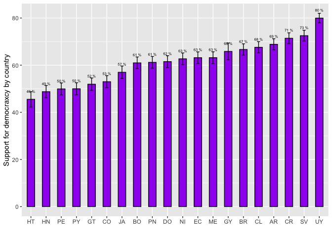

In the same way as above, inferences from this graph should be formalized by a inference test. To calculate if there are differences among these means, we can use the library survey. Before we have to fit the data.

Them we save the design in an object “design21”.

library(survey)
design21 = svydesign(ids = ~upm, strata = ~strata, weights = ~weight1500, nest=TRUE, data=lapop21)

For the calculation of the anova test we have to define a linear model, using support for democracy as dependent variable and “paises” as independent variable. We save this model in an object “model.anova”.

We can describe this model. These results show that the model has calculated different indicators for each country, assuming Mexico as the reference. So, we can see the mean of support for democracy for Mexico in the intercept of the model (63.2). Then, the value of each country corresponds to the difference of means with Mexico. For example, the value for Guatemala is -11.2, which us the difference in support for democracy between these two countries. This difference is equal to that obtained in the pairings above.

model.anova1=svyglm(ing4r ~ paises, design21)
summary(model.anova1)

## 
## Call:
## svyglm(formula = ing4r ~ paises, design = design21)
## 
## Survey design:
## svydesign(ids = ~upm, strata = ~strata, weights = ~weight1500, 
##     nest = TRUE, data = lapop21)
## 
## Coefficients:
##              Estimate Std. Error t value Pr(>|t|)    
## (Intercept)  63.19034    1.05514  59.888  < 2e-16 ***
## paisesGT    -11.24663    1.52445  -7.378 1.63e-13 ***
## paisesSV      9.32371    1.39984   6.661 2.75e-11 ***
## paisesHN    -14.42194    1.55413  -9.280  < 2e-16 ***
## paisesNI     -0.49551    1.58617  -0.312  0.75474    
## paisesCR      8.23324    1.43356   5.743 9.34e-09 ***
## paisesPN     -1.98863    1.47711  -1.346  0.17821    
## paisesCO    -10.19468    1.57860  -6.458 1.07e-10 ***
## paisesEC     -0.01354    1.47670  -0.009  0.99268    
## paisesBO     -2.21798    1.49084  -1.488  0.13683    
## paisesPE    -13.26646    1.52923  -8.675  < 2e-16 ***
## paisesPY    -13.21443    1.52474  -8.667  < 2e-16 ***
## paisesCL      4.39330    1.47807   2.972  0.00296 ** 
## paisesUY     16.78863    1.40219  11.973  < 2e-16 ***
## paisesBR      3.47217    1.64218   2.114  0.03449 *  
## paisesAR      5.66533    1.50069   3.775  0.00016 ***
## paisesDO     -1.67552    1.53256  -1.093  0.27427    
## paisesHT    -17.67392    1.80621  -9.785  < 2e-16 ***
## paisesJA     -6.19588    1.48863  -4.162 3.16e-05 ***
## paisesGY      2.64908    1.88539   1.405  0.16001    
## ---
## Signif. codes:  0 '***' 0.001 '**' 0.01 '*' 0.05 '.' 0.1 ' ' 1
## 
## (Dispersion parameter for gaussian family taken to be 2269.381)
## 
## Number of Fisher Scoring iterations: 2

To calculate the anova test for this model, we can use the command aov that uses as argument the object with the linear model. These results, in turn, are saved in an object “anova.w1”. We can present a summary of these results. Because the p-value (Pr>F) is lower than 0.05, we conclude than at least a pairing of means is different.

anova.w1=aov(model.anova1)
summary(anova.w1)

##                Df    Sum Sq Mean Sq F value Pr(>F)    
## paises         19   4325971  227683   100.3 <2e-16 ***
## Residuals   56733 128791904    2270                   
## ---
## Signif. codes:  0 '***' 0.001 '**' 0.01 '*' 0.05 '.' 0.1 ' ' 1
## 3898 observations deleted due to missingness

To evaluate all pairings, we can use the command TukeyHSD, using the results of object “anova.w1”. This command shows all pairings, taking into account a survey weight.

TukeyHSD(anova.w1)

##   Tukey multiple comparisons of means
##     95% family-wise confidence level
## 
## Fit: aov(formula = model.anova1)
## 
## $paises
##               diff           lwr          upr     p adj
## GT-ME -11.24663349 -15.655677424  -6.83758955 0.0000000
## SV-ME   9.32370920   5.033648918  13.61376949 0.0000000
## HN-ME -14.42193823 -18.811534518 -10.03234194 0.0000000
## NI-ME  -0.49550702  -4.859212929   3.86819888 1.0000000
## CR-ME   8.23324428   3.858787066  12.60770149 0.0000000
## PN-ME  -1.98862590  -6.291843413   2.31459161 0.9863114
## CO-ME -10.19467955 -14.562811779  -5.82654732 0.0000000
## EC-ME  -0.01354389  -4.369578999   4.34249122 1.0000000
## BO-ME  -2.21798400  -6.586486515   2.15051851 0.9630956
## PE-ME -13.26645772 -17.606017039  -8.92689840 0.0000000
## PY-ME -13.21443351 -17.587396711  -8.84147031 0.0000000
## CL-ME   4.39329834   0.009801469   8.77679521 0.0487209
## UY-ME  16.78862613  12.433679109  21.14357314 0.0000000
## BR-ME   3.47216639  -0.879888412   7.82422119 0.3367705
## AR-ME   5.66533305   1.311833838  10.01883226 0.0006962
## DO-ME  -1.67552383  -6.052604173   2.70155652 0.9986462
## HT-ME -17.67391966 -22.427556763 -12.92028255 0.0000000
## JA-ME  -6.19588247 -10.621731094  -1.77003384 0.0001269
## GY-ME   2.64908230  -2.790087949   8.08825255 0.9758382
## SV-GT  20.57034269  16.243887482  24.89679790 0.0000000
## HN-GT  -3.17530474  -7.600477394   1.24986791 0.5499872
## NI-GT  10.75112647   6.351634829  15.15061810 0.0000000
## CR-GT  19.47987776  15.069722063  23.89003347 0.0000000
## PN-GT   9.25800759   4.918505498  13.59750968 0.0000000
## CO-GT   1.05195394  -3.351928054   5.45583593 0.9999989
## EC-GT  11.23308960   6.841206255  15.62497294 0.0000000
## BO-GT   9.02864949   4.624400216  13.43289876 0.0000000
## PE-GT  -2.01982423  -6.395366771   2.35571830 0.9864787
## PY-GT  -1.96780002  -6.376473812   2.44087377 0.9907831
## CL-GT  15.63993183  11.220809489  20.05905416 0.0000000
## UY-GT  28.03525961  23.644455479  32.42606375 0.0000000
## BR-GT  14.71879988  10.330864324  19.10673543 0.0000000
## AR-GT  16.91196654  12.522598381  21.30133469 0.0000000
## DO-GT   9.57110966   5.158352045  13.98386728 0.0000000
## HT-GT  -6.42728617 -11.213794621  -1.64077772 0.0003460
## JA-GT   5.05075102   0.589615124   9.51188692 0.0092314
## GY-GT  13.89571579   8.427793840  19.36363774 0.0000000
## HN-SV -23.74564743 -28.052282062 -19.43901280 0.0000000
## NI-SV  -9.81921623 -14.099458682  -5.53897377 0.0000000
## CR-SV  -1.09046493  -5.381667804   3.20073795 0.9999971
## PN-SV -11.31233510 -15.530892583  -7.09377762 0.0000000
## CO-SV -19.51838875 -23.803143754 -15.23363375 0.0000000
## EC-SV  -9.33725309 -13.609674903  -5.06483128 0.0000000
## BO-SV -11.54169320 -15.826825695  -7.25656071 0.0000000
## PE-SV -22.59016692 -26.845789244 -18.33454461 0.0000000
## PY-SV -22.53814271 -26.827822586 -18.24846284 0.0000000
## CL-SV  -4.93041087  -9.230828409  -0.62999332 0.0075473
## UY-SV   7.46491692   3.193604505  11.73622934 0.0000001
## BR-SV  -5.85154281 -10.119906346  -1.58317928 0.0002124
## AR-SV  -3.65837615  -7.928212407   0.61146010 0.2122197
## DO-SV -10.99923303 -15.293109903  -6.70535616 0.0000000
## HT-SV -26.99762886 -31.674766017 -22.32049170 0.0000000
## JA-SV -15.51959167 -19.863171106 -11.17601223 0.0000000
## GY-SV  -6.67462690 -12.047067620  -1.30218618 0.0018013
## NI-HN  13.92643121   9.546429627  18.30643278 0.0000000
## CR-HN  22.65518250  18.264469524  27.04589549 0.0000000
## PN-HN  12.43331233   8.113570952  16.75305370 0.0000000
## CO-HN   4.22725868  -0.157152772   8.61167013 0.0747421
## EC-HN  14.40839434  10.036034968  18.78075371 0.0000000
## BO-HN  12.20395423   7.819173867  16.58873459 0.0000000
## PE-HN   1.15548051  -3.200464817   5.51142583 0.9999941
## PY-HN   1.20750472  -3.181719786   5.59672922 0.9999895
## CL-HN  18.81523657  14.415517326  23.21495581 0.0000000
## UY-HN  31.21056435  26.839289012  35.58183970 0.0000000
## BR-HN  17.89410462  13.525710681  22.26249855 0.0000000
## AR-HN  20.08727128  15.717438332  24.45710422 0.0000000
## DO-HN  12.74641440   8.353087991  17.13974081 0.0000000
## HT-HN  -3.25198143  -8.020581887   1.51661903 0.6487710
## JA-HN   8.22605576   3.784139434  12.66797209 0.0000000
## GY-HN  17.07102053  11.618768003  22.52327306 0.0000000
## CR-NI   8.72875130   4.363922079  13.09358052 0.0000000
## PN-NI  -1.49311888  -5.786548648   2.80031089 0.9996389
## CO-NI  -9.69917253 -14.057662794  -5.34068226 0.0000000
## EC-NI   0.48196313  -3.864403178   4.82832945 1.0000000
## BO-NI  -1.72247698  -6.081338349   2.63638439 0.9979430
## PE-NI -12.77095070 -17.100804427  -8.44109697 0.0000000
## PY-NI -12.71892649 -17.082258401  -8.35559457 0.0000000
## CL-NI   4.88880536   0.514916583   9.26269414 0.0112702
## UY-NI  17.28413315  12.938857351  21.62940895 0.0000000
## BR-NI   3.96767341  -0.374703728   8.31005055 0.1259014
## AR-NI   6.16084007   1.817015304  10.50466484 0.0000911
## DO-NI  -1.18001681  -5.547474942   3.18744133 0.9999921
## HT-NI -17.17841263 -21.923191235 -12.43363403 0.0000000
## JA-NI  -5.70037544 -10.116708120  -1.28404277 0.0008288
## GY-NI   3.14458932  -2.286840621   8.57601927 0.8809078
## PN-CR -10.22187018 -14.526226790  -5.91751357 0.0000000
## CO-CR -18.42792383 -22.797178232 -14.05866942 0.0000000
## EC-CR  -8.24678817 -12.603948568  -3.88962776 0.0000000
## BO-CR -10.45122828 -14.820852873  -6.08160368 0.0000000
## PE-CR -21.49970200 -25.840390879 -17.15901312 0.0000000
## PY-CR -21.44767779 -25.821761925 -17.07359365 0.0000000
## CL-CR  -3.83994594  -8.224561052   0.54466917 0.1797525
## UY-CR   8.55538185   4.199309259  12.91145444 0.0000000
## BR-CR  -4.76107789  -9.114259010  -0.40789677 0.0155842
## AR-CR  -2.56791123  -6.922536386   1.78671393 0.8626206
## DO-CR  -9.90876810 -14.286968333  -5.53056788 0.0000000
## HT-CR -25.90716393 -30.661832232 -21.15249563 0.0000000
## JA-CR -14.42912674 -18.856082917 -10.00217057 0.0000000
## GY-CR  -5.58416198 -11.024233474  -0.14409048 0.0365583
## CO-PN  -8.20605365 -12.503982118  -3.90812518 0.0000000
## EC-PN   1.97508201  -2.310551178   6.26071520 0.9867244
## BO-PN  -0.22935810  -4.527662902   4.06894670 1.0000000
## PE-PN -11.27783182 -15.546717510  -7.00894613 0.0000000
## PY-PN -11.22580761 -15.528645872  -6.92296934 0.0000000
## CL-PN   6.38192424   2.068381060  10.69546742 0.0000291
## UY-PN  18.77725203  14.492724809  23.06177924 0.0000000
## BR-PN   5.46079229   1.179204857   9.74237972 0.0010641
## AR-PN   7.65395895   3.370903343  11.93701456 0.0000000
## DO-PN   0.31310207  -3.993920367   4.62012451 1.0000000
## HT-PN -15.68529376 -20.374502185 -10.99608533 0.0000000
## JA-PN  -4.20725657  -8.563831600   0.14931847 0.0734775
## GY-PN   4.63770820  -0.745244795  10.02066120 0.2037244
## EC-CO  10.18113566   5.830325389  14.53194594 0.0000000
## BO-CO   7.97669555   3.613402944  12.33998816 0.0000000
## PE-CO  -3.07177817  -7.406092791   1.26253645 0.5747492
## PY-CO  -3.01975396  -7.387512573   1.34800466 0.6229728
## CL-CO  14.58797789  10.209673085  18.96628269 0.0000000
## UY-CO  26.98330568  22.633584804  31.33302655 0.0000000
## BR-CO  13.66684594   9.320020760  18.01367112 0.0000000
## AR-CO  15.86001260  11.511741273  20.20828393 0.0000000
## DO-CO   8.51915572   4.147275064  12.89103638 0.0000000
## HT-CO  -7.47924011 -12.228089850  -2.73039036 0.0000045
## JA-CO   3.99879708  -0.421909219   8.41950339 0.1375912
## GY-CO  12.84376185   7.408775084  18.27874862 0.0000000
## BO-EC  -2.20444011  -6.555622146   2.14674192 0.9638743
## PE-EC -13.25291383 -17.575036685  -8.93079098 0.0000000
## PY-EC -13.20088962 -17.556550081  -8.84522916 0.0000000
## CL-EC   4.40684223   0.040606356   8.77307810 0.0448627
## UY-EC  16.80217002  12.464597606  21.13974242 0.0000000
## BR-EC   3.48571028  -0.848958322   7.82037888 0.3217890
## AR-EC   5.67887694   1.342758137  10.01499574 0.0006061
## DO-EC  -1.66197994  -6.021773882   2.69781400 0.9987192
## HT-EC -17.66037577 -22.398100603 -12.92265093 0.0000000
## JA-EC  -6.18233858 -10.591092024  -1.77358513 0.0001216
## GY-EC   2.66262619  -2.762642826   8.08789521 0.9738312
## PE-BO -11.04847372 -15.383161517  -6.71378593 0.0000000
## PY-BO -10.99644951 -15.364578442  -6.62832057 0.0000000
## CL-BO   6.61128234   2.232608108  10.98995657 0.0000162
## UY-BO  19.00661013  14.656517399  23.35670285 0.0000000
## BR-BO   5.69015039   1.342953108  10.03734767 0.0006136
## AR-BO   7.88331705   3.534673745  12.23196035 0.0000000
## DO-BO   0.54246017  -3.829790456   4.91471080 1.0000000
## HT-BO -15.45593566 -20.205126003 -10.70674531 0.0000000
## JA-BO  -3.97789847  -8.398970653   0.44317372 0.1440493
## GY-BO   4.86706630  -0.568218073  10.30235068 0.1500265
## PY-PE   0.05202421  -4.287159033   4.39120746 1.0000000
## CL-PE  17.65975606  13.309957343  22.00955478 0.0000000
## UY-PE  30.05508385  25.734057628  34.37611007 0.0000000
## BR-PE  16.73862411  12.420512826  21.05673539 0.0000000
## AR-PE  18.93179077  14.612223726  23.25135781 0.0000000
## DO-PE  11.59093389   7.247601485  15.93426630 0.0000000
## HT-PE  -4.40746194  -9.130042777   0.31511891 0.1035032
## JA-PE   7.07057525   2.678099855  11.46305065 0.0000022
## GY-PE  15.91554002  10.503490773  21.32758927 0.0000000
## CL-PY  17.60773185  13.224607280  21.99085641 0.0000000
## UY-PY  30.00305964  25.648487361  34.35763191 0.0000000
## BR-PY  16.68659990  12.334920089  21.03827971 0.0000000
## AR-PY  18.87976656  14.526642215  23.23289090 0.0000000
## DO-PY  11.53890968   7.162202185  15.91561718 0.0000000
## HT-PY  -4.45948615  -9.212779943   0.29380765 0.0984075
## JA-PY   7.01855104   2.593071155  11.44403093 0.0000036
## GY-PY  15.86351581  10.424645598  21.30238602 0.0000000
## UY-CL  12.39532779   8.030177468  16.76047811 0.0000000
## BR-CL  -0.92113195  -5.283396818   3.44113292 0.9999999
## AR-CL   1.27203471  -3.091671188   5.63574061 0.9999740
## DO-CL  -6.06882217 -10.456054339  -1.68158999 0.0001708
## HT-CL -22.06721799 -26.830204404 -17.30423158 0.0000000
## JA-CL -10.58918080 -15.025069652  -6.15329196 0.0000000
## GY-CL  -1.74421604  -7.191559133   3.70312706 0.9998914
## BR-UY -13.31645974 -17.650034880  -8.98288459 0.0000000
## AR-UY -11.12329308 -15.458318787  -6.78826737 0.0000000
## DO-UY -18.46414995 -22.822856743 -14.10544317 0.0000000
## HT-UY -34.46254578 -39.199270206 -29.72582136 0.0000000
## JA-UY -22.98450859 -27.392186961 -18.57683023 0.0000000
## GY-UY -14.13954383 -19.563939233  -8.71514842 0.0000000
## AR-BR   2.19316666  -2.138953533   6.52528685 0.9641375
## DO-BR  -5.14769022  -9.503507286  -0.79187315 0.0045297
## HT-BR -21.14608605 -25.880151501 -16.41202059 0.0000000
## JA-BR  -9.66804886 -14.072869631  -5.26322808 0.0000000
## GY-BR  -0.82308409  -6.245157769   4.59898959 1.0000000
## DO-AR  -7.34085688 -11.698117107  -2.98359665 0.0000004
## HT-AR -23.33925271 -28.074646048 -18.60385936 0.0000000
## JA-AR -11.86121552 -16.267463402  -7.45496763 0.0000000
## GY-AR  -3.01625075  -8.439483860   2.40698236 0.9144352
## HT-DO -15.99839583 -20.755477611 -11.24131405 0.0000000
## JA-DO  -4.52035864  -8.949906856  -0.09081042 0.0392847
## GY-DO   4.32460613  -1.117574900   9.76678716 0.3444281
## JA-HT  11.47803719   6.676044811  16.28002957 0.0000000
## GY-HT  20.32300196  14.573604793  26.07239912 0.0000000
## GY-JA   8.84496477   3.363483391  14.32644614 0.0000020

For the 2018/19 round

To reproduce Figure 1.2 taking into account survey weights, we have to include a code that allows to make calculation including the variable “weight1500”. Some command in R allow to include a variable as weighted variable. For example, the library descr includes the command compmeans that we can use to calculate means (or proportions for a dummy variable) by groups of other variable, using a weighted variable. This command calculates the mean, the N and the standard deviation of each group. We can save this data in a new dataframe “df3”.

library(descr)
df3 = as.data.frame(compmeans(lapop18$ing4r, lapop18$paises, lapop18$weight1500, plot=F))

df3

In the same way as with the dataset for the 2021 round, we have to add vectors to this table.

varnames = c("media", "n", "sd")
colnames(df3) = varnames
df3$pais = row.names(df3)
df3$err.st = df3$sd/sqrt(df3$n)
df3$ci = df3$err.st*1.96
df3

With this new dataframe “df3”, which already includes the value of the confidence interval, we can replicate Figure 1.2, in a very similar way to the previous graph, but with the data considering survey weights.

fig1.2w <- ggplot(df3, aes(x=reorder(pais, media), y=media))+
  geom_bar(width=0.5, fill="purple", colour="black", stat="identity")+
  geom_errorbar(aes(ymin=media-ci, ymax=media+ci), width=0.2)+
  geom_text(aes(label=paste(round(media, 1), "%")), hjust=-0.8, size=2)+
  xlab("")+
  ylab("Support for democracy by country")+
  coord_flip()
fig1.2w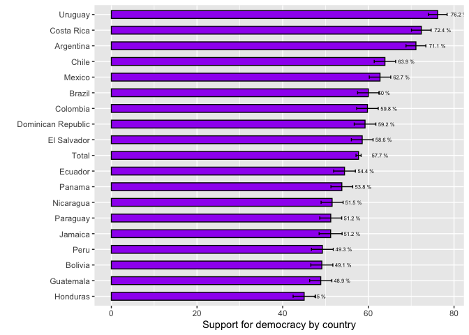

Other way to include the expansion factor is by using the library survey. The sample design is defined first.

library(survey)
design18 = svydesign(ids = ~upm, strata = ~estratopri, weights = ~weight1500, nest=TRUE, data=lapop18)

In the same way as with the 2021 round, we use a generalized linear model to calculate the ANOVA test.

model.anova2=svyglm(ing4r ~ paises, design18)

We describe this model to find that the p-value is lower than 0.05, so we affirm that at least one pairing is statistically different.

anova.w2=aov(model.anova2)
summary(anova.w2)

##                Df   Sum Sq Mean Sq F value Pr(>F)    
## paises         17  2022326  118960   50.25 <2e-16 ***
## Residuals   27068 64077761    2367                   
## ---
## Signif. codes:  0 '***' 0.001 '**' 0.01 '*' 0.05 '.' 0.1 ' ' 1
## 956 observations deleted due to missingness

We can also describe this model to calculate the weighted mean for Mexico in the intercept and the differences with respect to this reference country.

summary(model.anova2)

## 
## Call:
## svyglm(formula = ing4r ~ paises, design = design18)
## 
## Survey design:
## svydesign(ids = ~upm, strata = ~estratopri, weights = ~weight1500, 
##     nest = TRUE, data = lapop18)
## 
## Coefficients:
##                          Estimate Std. Error t value Pr(>|t|)    
## (Intercept)                62.723      1.246  50.342  < 2e-16 ***
## paisesGuatemala           -13.839      1.843  -7.508 1.10e-13 ***
## paisesEl Salvador          -4.157      1.777  -2.339   0.0195 *  
## paisesHonduras            -17.713      1.728 -10.249  < 2e-16 ***
## paisesNicaragua           -11.186      1.889  -5.922 4.05e-09 ***
## paisesCosta Rica            9.636      1.959   4.918 9.84e-07 ***
## paisesPanama               -8.917      1.854  -4.811 1.68e-06 ***
## paisesColombia             -2.933      1.738  -1.687   0.0918 .  
## paisesEcuador              -8.292      1.843  -4.499 7.42e-06 ***
## paisesBolivia             -13.582      1.855  -7.320 4.30e-13 ***
## paisesPeru                -13.458      1.828  -7.363 3.16e-13 ***
## paisesParaguay            -11.505      2.048  -5.619 2.34e-08 ***
## paisesChile                 1.148      1.703   0.674   0.5004    
## paisesUruguay              13.471      1.758   7.660 3.58e-14 ***
## paisesBrazil               -2.726      1.994  -1.367   0.1719    
## paisesArgentina             8.381      1.886   4.444 9.59e-06 ***
## paisesDominican Republic   -3.496      1.630  -2.145   0.0321 *  
## paisesJamaica             -11.534      1.819  -6.340 3.16e-10 ***
## ---
## Signif. codes:  0 '***' 0.001 '**' 0.01 '*' 0.05 '.' 0.1 ' ' 1
## 
## (Dispersion parameter for gaussian family taken to be 2365.803)
## 
## Number of Fisher Scoring iterations: 2

To evaluate all pairings we can use the command TukeyHSD of the object “anova.w2”.

TukeyHSD(anova.w2)

##   Tukey multiple comparisons of means
##     95% family-wise confidence level
## 
## Fit: aov(formula = model.anova2)
## 
## $paises
##                                        diff           lwr         upr     p adj
## Guatemala-Mexico               -13.83855232 -1.999973e+01  -7.6773698 0.0000000
## El Salvador-Mexico              -4.15651385 -1.037920e+01   2.0661694 0.6610397
## Honduras-Mexico                -17.71301987 -2.390599e+01 -11.5200532 0.0000000
## Nicaragua-Mexico               -11.18563360 -1.737547e+01  -4.9957931 0.0000000
## Costa Rica-Mexico                9.63632968  3.406062e+00  15.8665976 0.0000102
## Panama-Mexico                   -8.91695094 -1.506514e+01  -2.7687628 0.0000619
## Colombia-Mexico                 -2.93307293 -9.003533e+00   3.1373872 0.9695509
## Ecuador-Mexico                  -8.29184982 -1.446520e+01  -2.1184990 0.0003980
## Bolivia-Mexico                 -13.58196246 -1.964252e+01  -7.5214053 0.0000000
## Peru-Mexico                    -13.45836087 -1.964820e+01  -7.2685204 0.0000000
## Paraguay-Mexico                -11.50520478 -1.771397e+01  -5.2964408 0.0000000
## Chile-Mexico                     1.14790099 -4.987484e+00   7.2832859 0.9999999
## Uruguay-Mexico                  13.47052383  7.314362e+00  19.6266856 0.0000000
## Brazil-Mexico                   -2.72556793 -8.941800e+00   3.4906644 0.9886264
## Argentina-Mexico                 8.38061217  2.189731e+00  14.5714935 0.0003337
## Dominican Republic-Mexico       -3.49647245 -9.709496e+00   2.7165515 0.8866713
## Jamaica-Mexico                 -11.53435947 -1.789526e+01  -5.1734574 0.0000000
## El Salvador-Guatemala            9.68203847  3.470413e+00  15.8936643 0.0000081
## Honduras-Guatemala              -3.87446755 -1.005632e+01   2.3073886 0.7629806
## Nicaragua-Guatemala              2.65291872 -3.525806e+00   8.8316430 0.9909291
## Costa Rica-Guatemala            23.47488200  1.725566e+01  29.6941060 0.0000000
## Panama-Guatemala                 4.92160137 -1.215395e+00  11.0585978 0.3140674
## Colombia-Guatemala              10.90547939  4.846354e+00  16.9646043 0.0000001
## Ecuador-Guatemala                5.54670250 -6.155023e-01  11.7089073 0.1398794
## Bolivia-Guatemala                0.25658986 -5.792613e+00   6.3057932 1.0000000
## Peru-Guatemala                   0.38019145 -5.798533e+00   6.5589157 1.0000000
## Paraguay-Guatemala               2.33334754 -3.864334e+00   8.5310293 0.9980099
## Chile-Guatemala                 14.98645331  8.862283e+00  21.1106231 0.0000000
## Uruguay-Guatemala               27.30907615  2.116409e+01  33.4540608 0.0000000
## Brazil-Guatemala                11.11298439  4.907821e+00  17.3181477 0.0000001
## Argentina-Guatemala             22.21916449  1.603940e+01  28.3989315 0.0000000
## Dominican Republic-Guatemala    10.34207987  4.140131e+00  16.5440292 0.0000009
## Jamaica-Guatemala                2.30419285 -4.045892e+00   8.6542782 0.9987355
## Honduras-El Salvador           -13.55650602 -1.979966e+01  -7.3133528 0.0000000
## Nicaragua-El Salvador           -7.02911975 -1.326917e+01  -0.7890676 0.0104583
## Costa Rica-El Salvador          13.79284353  7.512687e+00  20.0729999 0.0000000
## Panama-El Salvador              -4.76043709 -1.095917e+01   1.4383001 0.3949847
## Colombia-El Salvador             1.22344092 -4.898210e+00   7.3450920 0.9999997
## Ecuador-El Salvador             -4.13533597 -1.035903e+01   2.0883595 0.6701887
## Bolivia-El Salvador             -9.42544861 -1.553728e+01  -3.3136176 0.0000112
## Peru-El Salvador                -9.30184702 -1.554190e+01  -3.0617949 0.0000296
## Paraguay-El Salvador            -7.34869093 -1.360751e+01  -1.0898671 0.0054118
## Chile-El Salvador                5.30441484 -8.816237e-01  11.4904534 0.2039911
## Uruguay-El Salvador             17.62703768  1.142039e+01  23.8336836 0.0000000
## Brazil-El Salvador               1.43094592 -4.835287e+00   7.6971784 0.9999980
## Argentina-El Salvador           12.53712603  6.296041e+00  18.7782107 0.0000000
## Dominican Republic-El Salvador   0.66004140 -5.603008e+00   6.9230912 1.0000000
## Jamaica-El Salvador             -7.37784562 -1.378762e+01  -0.9680718 0.0074803
## Nicaragua-Honduras               6.52738627  3.169675e-01  12.7378050 0.0274891
## Costa Rica-Honduras             27.34934955  2.109864e+01  33.6000626 0.0000000
## Panama-Honduras                  8.79606892  2.627164e+00  14.9649742 0.0000960
## Colombia-Honduras               14.77994694  8.688505e+00  20.8713886 0.0000000
## Ecuador-Honduras                 9.42117005  3.227186e+00  15.6151538 0.0000167
## Bolivia-Honduras                 4.13105741 -1.950515e+00  10.2126302 0.6311577
## Peru-Honduras                    4.25465900 -1.955760e+00  10.4650777 0.6156156
## Paraguay-Honduras                6.20781509 -2.146459e-02  12.4370948 0.0519723
## Chile-Honduras                  18.86092086  1.270478e+01  25.0170660 0.0000000
## Uruguay-Honduras                31.18354370  2.500669e+01  37.3603959 0.0000000
## Brazil-Honduras                 14.98745194  8.750729e+00  21.2241754 0.0000000
## Argentina-Honduras              26.09363204  1.988218e+01  32.3050882 0.0000000
## Dominican Republic-Honduras     14.21654742  7.983022e+00  20.4500731 0.0000000
## Jamaica-Honduras                 6.17866040 -2.022682e-01  12.5595890 0.0707772
## Costa Rica-Nicaragua            20.82196328  1.457435e+01  27.0695790 0.0000000
## Panama-Nicaragua                 2.26868265 -3.897084e+00   8.4344495 0.9984972
## Colombia-Nicaragua               8.25256067  2.164297e+00  14.3408240 0.0003239
## Ecuador-Nicaragua                2.89378378 -3.297074e+00   9.0846419 0.9779747
## Bolivia-Nicaragua               -2.39632886 -8.474718e+00   3.6820605 0.9965500
## Peru-Nicaragua                  -2.27272727 -8.480029e+00   3.9345740 0.9985861
## Paraguay-Nicaragua              -0.31957118 -6.545743e+00   5.9066005 1.0000000
## Chile-Nicaragua                 12.33353459  6.180534e+00  18.4865348 0.0000000
## Uruguay-Nicaragua               24.65615743  1.848244e+01  30.8298752 0.0000000
## Brazil-Nicaragua                 8.46006567  2.226447e+00  14.6936848 0.0003148
## Argentina-Nicaragua             19.56624577  1.335791e+01  25.7745850 0.0000000
## Dominican Republic-Nicaragua     7.68916115  1.458741e+00  13.9195810 0.0022475
## Jamaica-Nicaragua               -0.34872587 -6.726620e+00   6.0291687 1.0000000
## Panama-Costa Rica              -18.55328062 -2.475963e+01 -12.3469295 0.0000000
## Colombia-Costa Rica            -12.56940261 -1.869876e+01  -6.4400418 0.0000000
## Ecuador-Costa Rica             -17.92817950 -2.415946e+01 -11.6969006 0.0000000
## Bolivia-Costa Rica             -23.21829214 -2.933785e+01 -17.0987390 0.0000000
## Peru-Costa Rica                -23.09469055 -2.934231e+01 -16.8470748 0.0000000
## Paraguay-Costa Rica            -21.14153446 -2.740790e+01 -14.8751697 0.0000000
## Chile-Costa Rica                -8.48842869 -1.468210e+01  -2.2947606 0.0002512
## Uruguay-Costa Rica               3.83419415 -2.380056e+00  10.0484443 0.7849136
## Brazil-Costa Rica              -12.36189761 -1.863566e+01  -6.0881331 0.0000000
## Argentina-Costa Rica            -1.25571750 -7.504364e+00   4.9929295 0.9999997
## Dominican Republic-Costa Rica  -13.13280213 -1.940339e+01  -6.8622165 0.0000000
## Jamaica-Costa Rica             -21.17068915 -2.758783e+01 -14.7535518 0.0000000
## Colombia-Panama                  5.98387801 -6.203319e-02  12.0297892 0.0560683
## Ecuador-Panama                   0.62510112 -5.524111e+00   6.7743137 1.0000000
## Bolivia-Panama                  -4.66501152 -1.070098e+01   1.3709564 0.3827840
## Peru-Panama                     -4.54140993 -1.070718e+01   1.6243569 0.4764889
## Paraguay-Panama                 -2.58825383 -8.773018e+00   3.5965102 0.9931650
## Chile-Panama                    10.06485193  3.953755e+00  16.1759487 0.0000014
## Uruguay-Panama                  22.38747477  1.625552e+01  28.5194307 0.0000000
## Brazil-Panama                    6.19138302 -8.782402e-04  12.3836443 0.0500799
## Argentina-Panama                17.29756312  1.113075e+01  23.4643749 0.0000000
## Dominican Republic-Panama        5.42047849 -7.685621e-01  11.6095190 0.1742623
## Jamaica-Panama                  -2.61740853 -8.954887e+00   3.7200697 0.9941059
## Ecuador-Colombia                -5.35877689 -1.143027e+01   0.7127209 0.1640831
## Bolivia-Colombia               -10.64888953 -1.660567e+01  -4.6921137 0.0000001
## Peru-Colombia                  -10.52528794 -1.661355e+01  -4.4370246 0.0000002
## Paraguay-Colombia               -8.57213185 -1.467963e+01  -2.4646303 0.0001422
## Chile-Colombia                   4.08097392 -1.951917e+00  10.1138648 0.6386594
## Uruguay-Colombia                16.40359676  1.034958e+01  22.4576163 0.0000000
## Brazil-Colombia                  0.20750500 -5.907589e+00   6.3225985 1.0000000
## Argentina-Colombia              11.31368511  5.224364e+00  17.4030067 0.0000000
## Dominican Republic-Colombia     -0.56339952 -6.675232e+00   5.5484326 1.0000000
## Jamaica-Colombia                -8.60128654 -1.486339e+01  -2.3391862 0.0002385
## Bolivia-Ecuador                 -5.29011264 -1.135171e+01   0.7714838 0.1790452
## Peru-Ecuador                    -5.16651105 -1.135737e+01   1.0243470 0.2458653
## Paraguay-Ecuador                -3.21335496 -9.423133e+00   2.9964235 0.9429346
## Chile-Ecuador                    9.43975081  3.303339e+00  15.5761623 0.0000120
## Uruguay-Ecuador                 21.76237365  1.560519e+01  27.9195586 0.0000000
## Brazil-Ecuador                   5.56628189 -6.509637e-01  11.7835274 0.1462565
## Argentina-Ecuador               16.67246200  1.048056e+01  22.8643608 0.0000000
## Dominican Republic-Ecuador       4.79537737 -1.418660e+00  11.0094152 0.3856778
## Jamaica-Ecuador                 -3.24250965 -9.604402e+00   3.1193826 0.9500852
## Peru-Bolivia                     0.12360159 -5.954788e+00   6.2019909 1.0000000
## Paraguay-Bolivia                 2.07675768 -4.020901e+00   8.1744164 0.9994346
## Chile-Bolivia                   14.72986345  8.706937e+00  20.7527895 0.0000000
## Uruguay-Bolivia                 27.05248629  2.100840e+01  33.0965759 0.0000000
## Brazil-Bolivia                  10.85639453  4.751132e+00  16.9616574 0.0000001
## Argentina-Bolivia               21.96257464  1.588313e+01  28.0420239 0.0000000
## Dominican Republic-Bolivia      10.08549001  3.983494e+00  16.1874863 0.0000012
## Jamaica-Bolivia                  2.04760299 -4.204898e+00   8.3001038 0.9996615
## Paraguay-Peru                    1.95315609 -4.273016e+00   8.1793278 0.9998095
## Chile-Peru                      14.60626186  8.453262e+00  20.7592621 0.0000000
## Uruguay-Peru                    26.92888470  2.075517e+01  33.1026025 0.0000000
## Brazil-Peru                     10.73279294  4.499174e+00  16.9664121 0.0000003
## Argentina-Peru                  21.83897305  1.563063e+01  28.0473123 0.0000000
## Dominican Republic-Peru          9.96188842  3.731469e+00  16.1923082 0.0000037
## Jamaica-Peru                     1.92400140 -4.453893e+00   8.3018960 0.9998882
## Chile-Paraguay                  12.65310577  6.481069e+00  18.8251424 0.0000000
## Uruguay-Paraguay                24.97572861  1.878304e+01  31.1684192 0.0000000
## Brazil-Paraguay                  8.77963685  2.527227e+00  15.0320470 0.0001405
## Argentina-Paraguay              19.88581695  1.365861e+01  26.1130234 0.0000000
## Dominican Republic-Paraguay      8.00873233  1.759512e+00  14.2579527 0.0010806
## Jamaica-Paraguay                -0.02915469 -6.425416e+00   6.3671070 1.0000000
## Uruguay-Chile                   12.32262284  6.203504e+00  18.4417415 0.0000000
## Brazil-Chile                    -3.87346892 -1.005302e+01   2.3060804 0.7628142
## Argentina-Chile                  7.23271119  1.078664e+00  13.3867585 0.0053246
## Dominican Republic-Chile        -4.64437344 -1.082070e+01   1.5319485 0.4358766
## Jamaica-Chile                  -12.68226046 -1.900732e+01  -6.3572023 0.0000000
## Brazil-Uruguay                 -16.19609176 -2.239627e+01  -9.9959135 0.0000000
## Argentina-Uruguay               -5.08991165 -1.126467e+01   1.0848497 0.2661998
## Dominican Republic-Uruguay     -16.96699628 -2.316396e+01 -10.7700347 0.0000000
## Jamaica-Uruguay                -25.00488330 -3.135010e+01 -18.6596693 0.0000000
## Argentina-Brazil                11.10618010  4.871527e+00  17.3408328 0.0000001
## Dominican Republic-Brazil       -0.77090452 -7.027545e+00   5.4857359 1.0000000
## Jamaica-Brazil                  -8.80879154 -1.521230e+01  -2.4052802 0.0002302
## Dominican Republic-Argentina   -11.87708463 -1.810854e+01  -5.6456307 0.0000000
## Jamaica-Argentina              -19.91497165 -2.629388e+01 -13.5360669 0.0000000
## Jamaica-Dominican Republic      -8.03788702 -1.443828e+01  -1.6374901 0.0016139

The difference with respect to Mexico are equal to those reported in the generalized linear model. These differences include survey weights.